LeetFree - Leaked Interview questions from Google Facebook Amazon Microsoft LinkedIn

Question
Solution

Given a binary tree, return the values of its boundary in anti-clockwise direction starting from root. Boundary includes left boundary, leaves, and right boundary in order without duplicate nodes.

Left boundary is defined as the path from root to the left-most node. Right boundary is defined as the path from root to the right-most node. If the root doesn't have left subtree or right subtree, then the root itself is left boundary or right boundary. Note this definition only applies to the input binary tree, and not applies to any subtrees.

The left-most node is defined as a leaf node you could reach when you always firstly travel to the left subtree if exists. If not, travel to the right subtree. Repeat until you reach a leaf node.

The right-most node is also defined by the same way with left and right exchanged.

Example 1

Input:
  1
   \
    2
   / \
  3   4

Ouput:
[1, 3, 4, 2]

Explanation:
The root doesn't have left subtree, so the root itself is left boundary.
The leaves are node 3 and 4.
The right boundary are node 1,2,4. Note the anti-clockwise direction means you should output reversed right boundary.
So order them in anti-clockwise without duplicates and we have [1,3,4,2].

Example 2

Input:
    ____1_____
   /          \
  2            3
 / \          / 
4   5        6   
   / \      / \
  7   8    9  10  
       
Ouput:
[1,2,4,7,8,9,10,6,3]

Explanation:
The left boundary are node 1,2,4. (4 is the left-most node according to definition)
The leaves are node 4,7,8,9,10.
The right boundary are node 1,3,6,10. (10 is the right-most node).
So order them in anti-clockwise without duplicate nodes we have [1,2,4,7,8,9,10,6,3].

Solution
- Approach #1 Simple Solution [Accepted]
- Approach #2 Using PreOrder Traversal [Accepted]
\n

Solution

Approach #1 Simple Solution [Accepted]

Algorithm

One simple approach is to divide this problem into three subproblems- left boundary, leaves and right boundary.

Left Boundary: We keep on traversing the tree towards the left and keep on adding the nodes in the $res$ array, provided the current node isn\'t a leaf node. If at any point, we can\'t find the left child of a node, but its right child exists, we put the right child in the $res$ and continue the process. The following animation depicts the process.

\n\n

!?!../Documents/545_Boundary_Of_Binary_Tree1.json:1000,563!?!

Leaf Nodes: We make use of a recursive function addLeaves(res,root), in which we change the root node for every recursive call. If the current root node happens to be a leaf node, it is added to the $res$ array. Otherwise, we make the recursive call using the left child of the current node as the new root. After this, we make the recursive call using the right child of the current node as the new root. The following animation depicts the process.

\n\n

!?!../Documents/545_Boundary_Of_Binary_Tree2.json:1000,563!?!

Right Boundary: We perform the same process as the left boundary. But, this time, we traverse towards the right. If the right child doesn\'t exist, we move towards the left child. Also, instead of putting the traversed nodes in the $res$ array, we push them over a stack during the traversal. After the complete traversal is done, we pop the element from over the stack and append them to the $res$ array. The following animation depicts the process.

\n\n

!?!../Documents/545_Boundary_Of_Binary_Tree3.json:1000,563!?!

\n\n

Complexity Analysis

\n
Time complexity : $O(n)$ One complete traversal for leaves and two traversals upto depth of binary tree for left and right boundary.
\n
\n
Space complexity : $O(n)$ \n $res$ and $stack$ is used.
\n

Approach #2 Using PreOrder Traversal [Accepted]

Algorithm

Before we dive into this approach, let\'s look at the preorder traversal of a simple Binary Tree as shown below:

Preorder Traversal

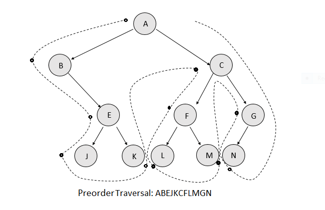
From the above figure, we can observe that our problem statement is very similar to the Preorder traversal. Actually, the order of traversal is the same(except for the right boundary nodes, for which it is the reverse), but we need to selectively include the nodes in the return result list. Thus, we need to include only those nodes in the result, which are either on the left boundary, the leaves or the right boundary.

In order to distinguish between the various kinds of nodes, we make use of a $flag$ as follows:

\n
Flag=0: Root Node.
\n
\n
Flag=1: Left Boundary Node.
\n
\n
Flag=2: Right Boundary Node.
\n
\n
Flag=3: Others(Middle Node).
\n

We make use of three lists $\\text{left_boundary}$ , $\\text{right_boundary}$ , $\\text{leaves}$ to store the appropriate nodes and append the three lists at the end.

We go for the normal preorder traversal, but while calling the recursive function for preorder traversal using the left child or the right child of the current node, we also pass the $flag$ information indicating the type of node that the current child behaves like.

For obtaining the flag information about the left child of the current node, we make use of the function leftChildFlag(node, flag). In the case of a left child, the following cases are possible, as can be verified by looking at the figure above:

\n
The current node is a left boundary node: In this case, the left child will always be a left boundary node. e.g. relationship between E & J in the above figure.
\n
\n
The current node is a root node: In this case, the left child will always be a left boundary node. e.g. relationship between A & B in the above figure.
\n
\n
The current node is a right boundary node: In this case, if the right child of the current node doesn\'t exist, the left child always acts as the right boundary node. e.g. G & N. But, if the right child exists, the left child always acts as the middle node. e.g. C & F.
\n

Similarly, for obtaining the flag information about the right child of the current node, we make use of the function rightChildFlag(node, flag). In the case of a right child, the following cases are possible, as can be verified by looking at the figure above:

\n
The current node is a right boundary node: In this case, the right child will always be a right boundary node. e.g. relationship between C & G in the above figure.
\n
\n
The current node is a root node: In this case, the right child will always be a left boundary node. e.g. relationship between A & C in the above figure.
\n
\n
The current node is a left boundary node: In this case, if the left child of the current node doesn\'t exist, the right child always acts as the left boundary node. e.g. B & E. But, if the left child exists, the left child always acts as the middle node.
\n

Making use of the above information, we set the $flag$ appropriately, which is used to determine the list in which the current node has to be appended.

\n\n

Complexity Analysis

\n
Time complexity : $O(n)$ One complete traversal of the tree is done.
\n
\n
Space complexity : $O(n)$ The recursive stack can grow upto a depth of $n$ . Further, $\\text{left_boundary}$ , $\\text{right_boundary}$ and $\\text{leaves}$ combined together can be of size $n$ .
\n

Analysis written by: @vinod23

545. Boundary of Binary Tree

Solution

Approach #1 Simple Solution [Accepted]

Approach #2 Using PreOrder Traversal [Accepted]