All leaked interview problems are collected from Internet.
634. Find the Derangement of An Array
In combinatorial mathematics, a derangement is a permutation of the elements of a set, such that no element appears in its original position.
There's originally an array consisting of n integers from 1 to n in ascending order, you need to find the number of derangement it can generate.
Also, since the answer may be very large, you should return the output mod 109 + 7.
Example 1:
Input: 3
Output: 2
Explanation: The original array is [1,2,3]. The two derangements are [2,3,1] and [3,1,2].
Note:
n is in the range of [1, 106].
b'
Solution
\n\n
Approach #1 Brute Force [Time Limit Exceeded]
\nThe simplest solution is to consider every possible permutation of the given numbers from to and count the number of permutations which are dereangements of the \noriginal arrangement.
\nComplexity Analysis
\n- \n
- \n
Time complexity : . permutations are possible for numbers. For each permutation, we need to traverse over the whole arrangement to check if it \nis a derangement or not, which takes time.
\n \n - \n
Space complexity : . Each permutation would require space to be stored.
\n \n
\n
Approach #2 Using Recursion [Stack Overflow]
\nAlgorithm
\nIn order to find the number of derangements for numbers, firstly we can consider the the original array to be \n[1,2,3,...,n]. Now, in order to generate the derangements of this array, assume that firstly, we move the number 1 from \nits original position and place at the place of the number . But, now, this position can be chosen \nin ways. Now, for placing the number we have got two options:
- \n
- \n
We place at the place of : By doing this, the problem of finding the derangements reduces to finding the derangements of the \nremaining numbers, since we\'ve got numbers and places, such that every number can\'t be placed at exactly one position.
\n \n - \n
We don\'t place at the place of : By doing this, the problem of finding the derangements reduces to finding the \nderangements for the elements(except 1). This is because, now we\'ve got elements and these elements can\'t be placed at \nexactly one location(with not being placed at the first position).
\n \n
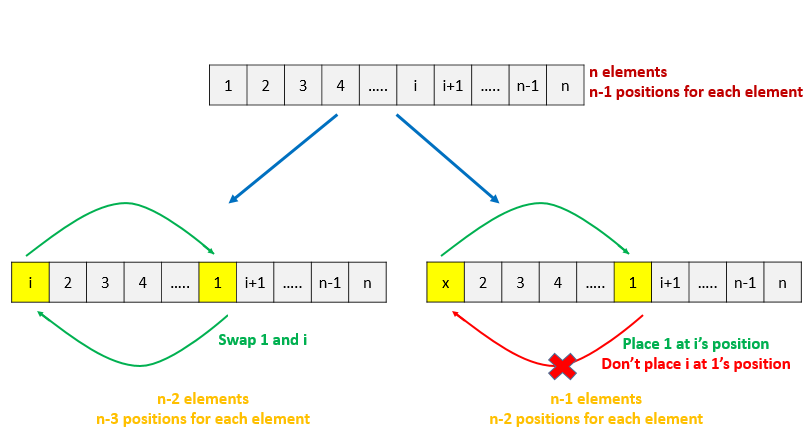
Based, on the above discussion, if represents the number of derangements for elements, it can be obtained as:
\n\n\n
\nThis is a recursive equation and can thus, be solved easily by making use of a recursive function.
\nBut, if we go with the above method, a lot of duplicate function calls wiil be made, with the same parameters being passed. This is because the same state can be reached through various paths in the recursive tree. In order to avoid these duplicate calls, we can store the result of a function call, once its made, \ninto a memoization array. Thus, whenever the same function call is made again, we can directly return the result from this memoization array. \nThis helps to prune the search space to a great extent.
\n\nComplexity Analysis
\n- \n
- \n
Time complexity : . array of length is filled once only.
\n \n - \n
Space complexity : . array of length is used.
\n \n
\n
Approach #3 Dynamic Programming [Accepted]:
\nAlgorithm
\nAs we\'ve discussed above, the recursive formula for finding the derangements for elements is given by:
\n\n\n
\nFrom this expression, we can see that the result for derangements for numbers depends only on the result of the derangments \nof numbers lesser than . Thus, we can solve the given problem by making use of Dynamic Programming.
\nThe equation for Dynamic Programming remains identical to the recursive equation.
\n\n\n
\nHere, is used to store the number of derangements for elements. We start filling the array from and move towards the larger values of . At the end, the value of \n gives the required result.
\nThe following animation illustrates the filling process.
\n!?!../Documents/634_Find_Derangements.json:1000,563!?!
\n\nComplexity Analysis
\n- \n
- \n
Time complexity : . Single loop upto is required to fill the array of size .
\n \n - \n
Space complexity : . array of size is used.
\n \n
\n
Approach #4 Constant Space Dynamic Programming [Accepted]:
\nAlgorithm
\nIn the last approach, we can easily observe that the result for depends only on the previous two elements, and \n. Thus, instead of maintaining the entire 1-D array, we can just keep a track of the last two values required to calculate the \nvalue of the current element. By making use of this observation, we can save the space required by the array in the last approach.
\n\nComplexity Analysis
\n- \n
- \n
Time complexity : . Single loop upto is required to find the required result.
\n \n - \n
Space complexity : . Constant extra space is used.
\n \n
\n
Approach #5 Using Formula [Accepted]:
\nAlgorithm
\nBefore discussing this approach, we need to look at some preliminaries.
\nIn combinatorics (combinatorial mathematics), the inclusion\xe2\x80\x93exclusion principle is a counting \ntechnique which generalizes the familiar method of obtaining the number of elements in the union of two \nfinite sets; symbolically expressed as
\n\n\n
\nwhere and are two finite sets and indicates the cardinality of a set \n(which may be considered as the number of elements of the set, if the set is finite).
\n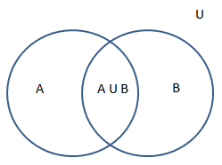
The formula expresses the fact that the sum of the sizes of the two sets may be too large since\n some elements may be counted twice. The double-counted elements are those in the intersection of \n the two sets and the count is corrected by subtracting the size of the intersection.
\nThe principle is more clearly seen in the case of three sets, which for the sets , and is given by
\n\n.
\nThis formula can be verified by counting how many times each region in the \nVenn diagram figure shown below.
\n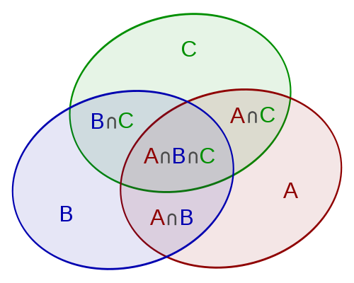
In this case, \nwhen removing the contributions of over-counted elements, the number of elements in the mutual \nintersection of the three sets has been subtracted too often, so must be added back in to get the correct total.
\nIn its general form, the principle of inclusion\xe2\x80\x93exclusion states that for finite sets , one\n has the identity
\n\n\n
\n\n\n
\nBy applying De-Morgan\'s law to the above equation, we can obtain
\n\n\n\n
\nHere, represents the universal set containing all of the and denotes the complement of in .
\nNow, let denote the set of permutations which leave in its natural position. Thus, the number of permutations in which \nthe element remains at its natural position is . Thus, the component above \nbecomes . Here, represents the number of ways of choosing 1 element out of elements.
\nMaking use of this notation, the required number of derangements can be denoted by term.
\nThis is the same term which has been expanded in the last equation. Putting appropriate values of the elements, we can expand the above equation as:
\n\n\n\n
\n\n\n
\nWe can make use of this formula to obtain the required number of derangements.
\n\nComplexity Analysis
\n- \n
- \n
Time complexity : . Single loop upto is used.
\n \n - \n
Space complexity : . Constant space is used.
\n \n
\n
Analysis written by: @vinod23
\n